Active Learning Overview: Strategies and Uncertainty Measures
Active Learning Overview: Strategies and Uncertainty Measures
1. Active Learning
· Active learning is the name used for the process of prioritizing the data which needs to be labelled in order to have the highest impact to training a supervised model.
· Active learning is a strategy in which the learning algorithm can interactively query a user (teacher or oracle) to label new data points with the true labels. The process of active learning is also referred to as optimal experimental design.
· Active learning is motivated by the understanding that not all labelled examples are equally important.
· Active Learning is a methodology that can sometimes greatly reduce the amount of labeled data required to train a model. It does this by prioritizing the labeling work for the experts.
- Active Learning Allows to reduce cost while improving accuracy.
- Is an enhancement on top of your existing model.
- It is a strategy/algorithm, not a model.
- But can be hard. “Active learning is easy to understand, not easy to execute on”
The key idea behind active learning is that a machine learning algorithm can achieve greater accuracy with fewer training labels if it is allowed to choose the data from which it learns. — Active Learning Literature Survey, Burr Settles
Instead of collecting all the labels for all the data at once, Active Learning prioritizes which data the model is most confused about and requests labels for just those. The model then trains a little on that small amount of labeled data, and then again asks for some more labels for the most confusing data.
By prioritizing the most confusing examples, the model can focus the experts on providing the most useful information. This helps the model learn faster, and lets the experts skip labeling data that wouldn’t be very helpful to the model. The result is that in some cases we can greatly reduce the number of labels we need to collect from experts and still get a great model. This means time and money savings for machine learning projects!
2. Active learning strategy
Steps for active learning
There are multiple approaches studied in the literature on how to prioritize data points when labelling and how to iterate over the approach. We will nevertheless only present the most common and straightforward methods.
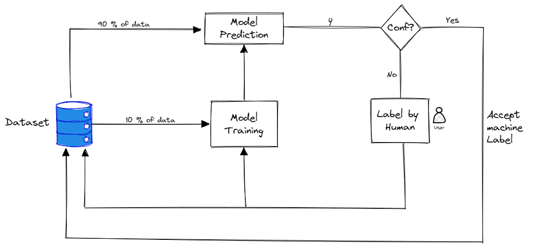
The steps to use active learning on an unlabeled data set are:
- The first thing which needs to happen is that a very small subsample of this data needs to be manually labelled.
- Once there is a small amount of labelled data, the model needs to be trained on it. The model is of course not going to be great, but will help us get some insight on which areas of the parameter space need to be labelled first to improve it.
- After the model is trained, the model is used to predict the class of each remaining unlabeled data point.
- A score is chosen on each unlabeled data point based on the prediction of the model. In the next subsection, we will present some of the possible scores most commonly used.
- Once the best approach has been chosen to prioritize the labelling, this process can be iteratively repeated: a new model can be trained on a new labelled data set, which has been labelled based on the priority score. Once the new model has been trained on the subset of data, the unlabelled data points can be run through the model to update the prioritization scores to continue labelling. In this way, one can keep optimizing the labelling strategy as the models become better and better.
General Strategy of AL / Image by Author
2.1 Active Learning Approach #1 : Streaming
In stream-based active learning, the set of all training examples is presented to the algorithm as a stream. Each example is sent individually to the algorithm for consideration. The algorithm must make an immediate decision on whether to label or not label this example. Selected training examples from this pool are labelled by the oracle, and the label is immediately received by the algorithm before the next example is shown for consideration.
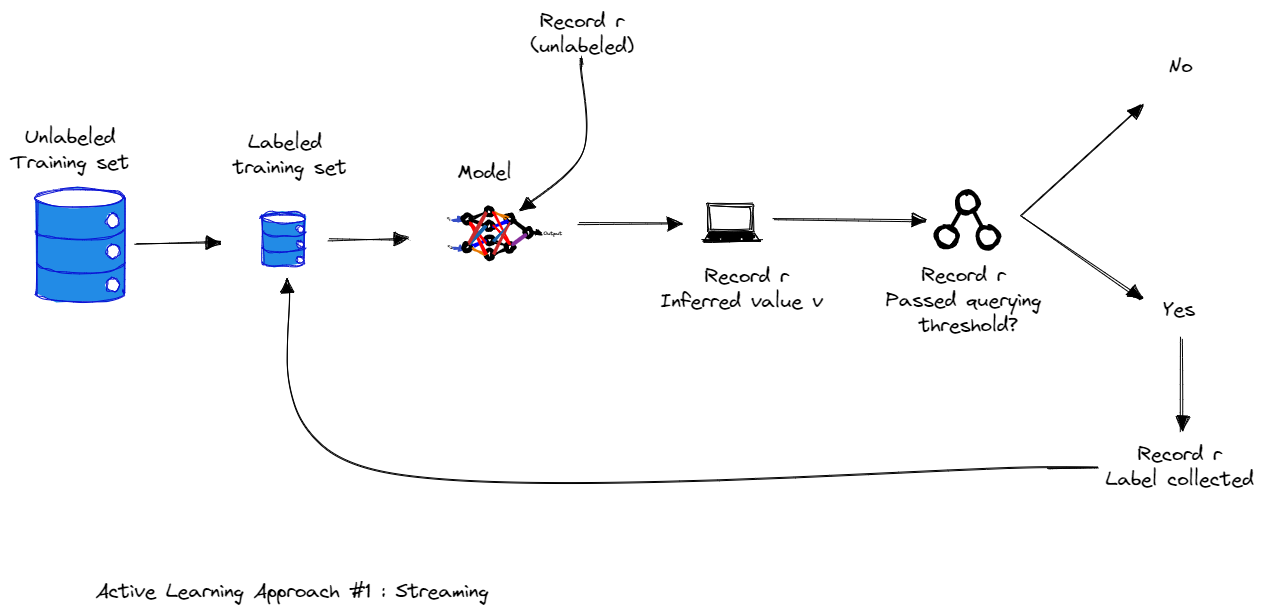 Image by Author
2.2. Active Learning Approach #2: Pooling
In pool-based sampling, training examples are chosen from a large pool of unlabeled data. Selected training examples from this pool are labelled by the oracle.
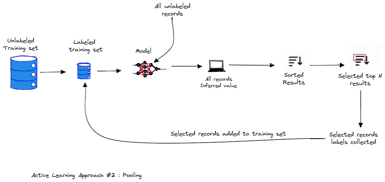 Image by Author
2.3 Active Learning Approach #3: Query by Committee
Query by committee in words is the use of multiple models instead of one.
An alternative approach, called Query by Committee, maintains a collection of models (the committee) and selecting the most “controversial” data point to label next, that is one where the models disagreed on. Using such a committee may allow us to overcome the restricted hypothesis a single model can express, though at the onset of a task we still have no way of knowing what hypothesis we should be using.
3. Uncertainty Measures
The process of identifying the most valuable examples to label next is referred to as “sampling strategy” or “query strategy”. The scoring function in the sampling process is named “acquisition function”. Data points with higher scores are expected to produce higher value for model training if they get labeled. There are different sampling strategies such as Uncertainty Sampling, Diversity Sampling, Expected Model Change…, In this article we will focus only on the uncertainty measures which is the most used strategy.
Uncertainty sampling is a set of techniques for identifying unlabeled items that are near a decision boundary in your current machine learning model. Although it is easy to identify when a model is confident — there is one result with very high confidence — you have many ways to calculate uncertainty, and your choice will depend on your use case and what is the most effective for your particular data.
The most informative examples are the ones that the classifier is the least certain about.
The intuition here is that the examples for which the model has the least certainty will likely be the most difficult examples — specifically, the examples that lie near the class boundaries. The learning algorithm will gain the most information about the class boundaries by observing the difficult examples.
Let’s take a concrete example, say you are trying to build a multi class classification to distinguish between 3 classes Cat, Dog, Horse. The model might give us a prediction like the following:
This output is most likely from softmax, which converts the logits to a 0–1 range of scores using the exponents.
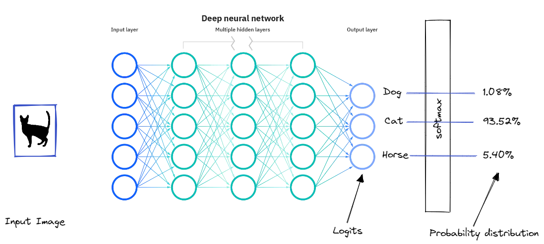 Image by Author
3.1. Least confidence:
Least confidence takes the difference between 1 (100% confidence) and the most confidently predicted label for each item.
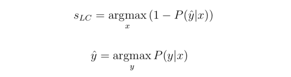
Although you can rank order by confidence alone, it can be useful to convert the uncertainty scores to a 0–1 range, where 1 is the most uncertain score. In that case, we have to normalize the score. We subtract the value from 1, multiply the result by n/(1-n) with n being the number of labels. We do this because the minimum confidence can never be less than the one divided by the number of labels, which is when all labels have the same predicted confidence.
Let’s apply this to our example, the uncertainty score would be :
(1–0.9352) * (3/2) = 0.0972.
Least confidence is the simplest and most used method, it gives you ranked order of predictions where you will sample items with the lowest confidence for their predicted label.
3.2. Margin of confidence sampling
The most intuitive form of uncertainty sampling is the difference between the two most confident predictions. That is, for the label that the model predicted, how much more confident was it than for the next-most-confident label? This is defined as :

Again, we can convert this to a 0–1 range. We have to subtract from 1.0 again, but the maximum possible score is already 1, so there is no need to multiply by any factor.
Let’s apply margin of confidence sampling to our example data. “Cat” and “Horse” are the most-confident and second-most-confident prediction. Using our example, this uncertainty score would be 1.0 — (0.9352–0.0540) = 0.1188.
3.3. Ratio sampling
Ratio of confidence is a slight variation on margin of confidence, looking at the ratio between the top two scores instead of the difference.

Now let’s plug in our numbers again: 0.9352 / 0.0540 = 17.3185.
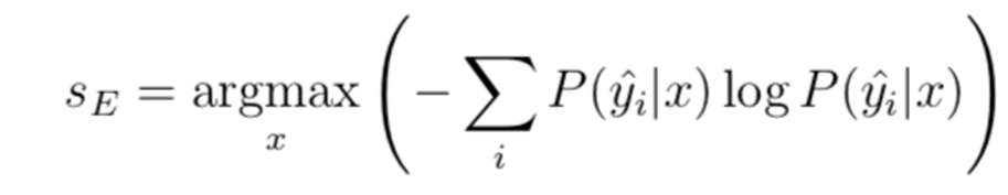
3.4. Entropy Sampling
Entropy applied to a probability distribution involves multiplying each probability by its own log and taking the negative sum:
Let’s calculate the entropy on our example data:
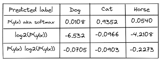 Table by Author
Summing the numbers and negating them returns 0 — SUM(–0.0705, –0.0903, –0.2273) = 0.3881
Dividing by the log of the number of labels returns 0.3881/ log2(3) = 0.6151
4. Closing up
Most of the focus of the machine learning community is in creating better algorithms for learning from data. But getting useful annotated datasets is difficult. Really difficult. It can be expensive, time-consuming, and you still end up with problems like annotations missing from some categories. Active Learning is a great building block for this, and is under utilized in my opinion.